Quick Start Guide
Get up and running with PermeableDT in minutes! This guide will walk you through your first simulation, calibration, and forecasting example.
Prerequisite
permeabledt installed (Installation Guide)
Basic Python knowledge
Your data files ready (Examples or Data Preparation)
1. Water Flow Simulation
Step 1: Download the input_parameters.ini and rainfall.dat from the examples folder on the permeabledt/examples
Step 2: Import the modules and declare the files
import permeabledt as pdt
import permeabledt.plots as plots

# Load parameters from INI file
setup = pdt.read_setup_file("input_parameters.ini")
params = pdt.initialize_parameters(setup)
rainfall_file = 'rainfall.dat'
output_path = "test_plot.png"
Step 3: Run Simulation
# Run the simulation
# # run the simulation
data, mb = pdt.run_simulation(params,
                              rainfall_file,
                              rainfall_unit='in',
                              verbose=True,
                              plot_outflow=True,
                              output_path=output_path)
You can analyze your raw results on the data pandas.DataFrame and visualize the plot on the output path
2. Calibration and validation
Step 1: Organize the folders and download the input files from the permeabledt/examples/calibration_validation
Make sure that your input_parameters.ini has a section [CALIBRATION]. Inside this section, input all the parameters to be calibrated as a lower bound and upper bound. Also include the pop and gen parameters for population size and generations respectively.
[CALIBRATION]
cd_min = 0.3
cd_max = 1.0
gama_min = 1
gama_max = 10
hpipe_min = 0
hpipe_max = 0.1
eta_min = 0.3
eta_max = 1.0
;population size (integer)
pop = 100
;generation size (integer)
gen = 50
Step 2: Make sure to have all the libraries installed
pip install 'permeabledt[calib]'
Step 3: Import the libraries, declare the correct paths and run the calibration:
import permeabledt as gdt
from permeabledt import plots
import os
from pathlib import Path
import pandas as pd

print(os.getcwd())

base_dir = os.getcwd()

setup_file = os.path.join(base_dir, "input", "input_parameters.ini")
print(setup_file)

calibration_path = Path(os.path.join(base_dir, "input", "calibration"))
calibration_rainfall = sorted(calibration_path.glob('*.dat'))
calibration_observed_data = sorted(calibration_path.glob('*.csv'))

# Output files
output_setup_file = os.path.join(base_dir, "output", f"calibrated_parameters.ini")
logbook_path = os.path.join(base_dir, "output", "calibration_logbook.csv")

# # Run calibration
best_params, calibrated_setup, logbook = gdt.run_calibration(
    calibration_rainfall=calibration_rainfall,
    calibration_observed_data=calibration_observed_data,
    setup_file=setup_file,
    output_setup_file=output_setup_file,
    logbook_output_path=logbook_path,
    seed=2025  # For reproducibility
)

# Plot the calibration events
setup_calibration = gdt.read_setup_file(output_setup_file)
parameters = gdt.initialize_parameters(setup_calibration)

# Plot comparisons
_, _, metrics_calib = plots.plot_event_comparison(
    rainfall_files=calibration_rainfall,
    observed_files=calibration_observed_data,
    parameters=parameters,
    rainfall_unit='in',
    output_folder= os.path.join(base_dir, "output", 'calibration_plots'),
    ncols=1  # Number of columns in the grid
)
Step 4: Run the validation
In the same way as the calibration:
validation_path = Path(os.path.join(base_dir, "input", "validation"))
validation_rainfall = sorted(validation_path.glob('*.dat'))
validation_observed_data = sorted(validation_path.glob('*.csv'))

_, _, metrics_valid = plots.plot_event_comparison(
    rainfall_files=validation_rainfall,
    observed_files=validation_observed_data,
    parameters=parameters,
    rainfall_unit='in',
    output_folder= os.path.join(base_dir, "output", 'validation_plots'),
    ncols=1  # Number of columns in the grid
)

df_calib = pd.DataFrame(metrics_calib).T
df_valid = pd.DataFrame(metrics_valid).T

print(df_calib.to_string())
print(df_valid.to_string())
3. Download Forecast Rainfall (HRRR):
This is an optional module from the permeabledt, however, if you want to compare your particle filtering model with historical forecasts, this module is useful to download the historical forecast files. To download real-time forecasts, consult the Herbie documentation.
The input files and folder organization necessary to run the code can be found in permeabledt/examples/download_forecast_rainfall
Run the HRRR code to download the data for the specific coordinate:
from permeabledt import download_HRRR_historical_forecast
import pandas as pd
import os
import permeabledt as pdt

base_dir = os.getcwd()
rainfall_file = os.path.join(base_dir, "input", "event_00_rainfall.dat")
rainfall_obs = pdt.water_flow_module.read_rainfall_dat_file(rainfall_file)
rainfall_obs['date'] = pd.to_datetime(rainfall_obs['date'])
start_date = rainfall_obs['date'][0].floor("h")
end_date = rainfall_obs['date'][len(rainfall_obs) - 1].ceil("h")
output_dir = os.path.join(base_dir, 'output', str(start_date.date()))
# Permeable Pavement Site - San Antonio, TX coordinates
lat = 29.629438
lon = -98.476345

# Initialize downloader
downloader = download_HRRR_historical_forecast.HRRRAccumulatedPrecipitationDownloader(lat, lon, timezone='US/Central')

# Explore available variables
downloader.explore_precipitation_variables(
    sample_date=start_date,
    product='subh'
)

# Download accumulated precipitation data
forecast_dataframes = downloader.download_date_range(
    start_date=start_date,
    end_date=end_date,
    forecast_hours=6
)

# Display results
print("\n" + "=" * 80)
print("RESULTS SUMMARY")
print("=" * 80)

all_data = []
for i, df in enumerate(forecast_dataframes):
    if df is not None and len(df) > 0:
        model_run = df['model_run'].iloc[0]
        print(f"\nForecast {i + 1}: Model run at {model_run} UTC")
        print(f"Total points: {len(df)}")
        print(f"Variables used: {df['variable_used'].unique()}")
        print(f"\nFirst 10 rows:")
        print(df[['forecast_time_local', 'precipitation_mm', 'step_range']].head(10))

        # Collect all data
        all_data.append(df)

    # Save results
    if forecast_dataframes:
        downloader.save_to_csv(forecast_dataframes, output_dir)

        # Create a combined file with all forecasts
        if all_data:
            combined_df = pd.concat(all_data, ignore_index=True)
            combined_df = combined_df.sort_values(['forecast_time', 'model_run']).reset_index(drop=True)
            combined_df.to_csv(os.path.join(f'output\hrrr_all_accumulated_forecasts_{start_date.date()}.csv'), index=False)
            print(f"\nSaved combined file: output\\hrrr_all_accumulated_forecasts_{start_date.date()}.csv")

            # Show summary statistics
            print(f"\nSummary Statistics:")
            print(f"Total forecast points: {len(combined_df)}")
            print(f"Time range: {combined_df['forecast_time_local'].min()} to {combined_df['forecast_time_local'].max()}")
            print(f"Total precipitation: {combined_df['precipitation_mm'].sum():.2f} mm")
            print(f"Max 15-min precipitation: {combined_df['precipitation_mm'].max():.2f} mm")


# Plot and extract the metrics to compare with the observed rainfall
metrics, _ = downloader.compare_with_observed(
    forecast_dir=output_dir,
    observed=rainfall_obs,
    cumulative=False,
    plot=True,
    output_dir = rf'output\plots\{str(start_date.date())}'
)
4. Particle Filter
This is a simple approach to incorporate assimilated data to the particle filter, and collect the results. In this approach, we will run for a single time-step. For online estimation refer to the pypfilt Documentation
Please, address to the permeabledt/examples/particle_filter to download the input files and folder organization.
Step 1: Define functions that will be used for the particle filtering input data processing and post-processing (plots)
import pypfilt
import permeabledt as pdt
import pandas as pd
import datetime as dt
import numpy as np
import os
import pytz
from pathlib import Path
import matplotlib.pyplot as plt


def run_pp_forecast(forecast_time, scenario_file, filename=None):
    instances = list(pypfilt.load_instances(scenario_file))
    instance = instances[0]

    ctx = instance.build_context()
    # Run the forecast and return both the results and the final context object
    results = pypfilt.forecast(ctx, [forecast_time], filename=filename)
    return results, ctx


def create_outflow_file(observed_outflow_file, output_dir="", forecast=False, forecast_time=None):
    cfs_to_m3s = 0.028316847
    df = pd.read_csv(observed_outflow_file, parse_dates=[0]).dropna()
    if forecast:
        df.set_index('date', inplace=True)
        df = df.resample("15min").mean().reset_index()

        # Select the data that has been observed up to the current forecast time
        forecast_date = df['date'][0] + dt.timedelta(
            minutes=forecast_time * 15)  # Converting from 1-minute to 15-minute timestep
        df = df[df['date'] <= forecast_date]

    df.columns = ['time', 'value']
    df['time'] = np.arange(len(df), dtype=float)
    df['value'] = df['value'] * cfs_to_m3s

    df.to_csv(f'{output_dir}\\observed_outflow.ssv', sep=" ", index=False)
    return df


def prepare_forecast_rainfall_file(forecast_time, HRRR_folder, rainfall_file, output_folder):
    # Converting the forecast time in 15-minutes time step to minute time step, as the original data is in minutes
    forecast_time = forecast_time * 15

    # Load and process observed rainfall
    obs_rainfall = pdt.water_flow_module.read_rainfall_dat_file(rainfall_file)
    obs_rainfall['date'] = pd.to_datetime(obs_rainfall['date']).dt.tz_localize(None)
    obs_rainfall.set_index('date', inplace=True)
    obs_rainfall = obs_rainfall.resample("15min").sum().reset_index()

    # Get forecast date (tz-naive), rounded to ceiling hour
    forecast_date = obs_rainfall['date'][0] + dt.timedelta(minutes=forecast_time)
    forecast_date = pd.Timestamp(forecast_date).ceil('h').to_pydatetime()

    # Convert to UTC for filename lookup
    cdt = pytz.timezone('America/Chicago')
    forecast_date_cdt = cdt.localize(forecast_date)
    forecast_date_utc = forecast_date_cdt.astimezone(pytz.UTC)

    file_timestamp = forecast_date_utc.strftime('%Y%m%d_%H%M_UTC')
    forecast_filename = f"hrrr_accumulated_{file_timestamp}.csv"
    forecast_path = os.path.join(HRRR_folder, forecast_filename)

    if not os.path.exists(forecast_path):
        raise FileNotFoundError(f"Forecast file not found: {forecast_path}")

    # Load and prepare forecast data
    forecast_df = pd.read_csv(forecast_path, parse_dates=['forecast_time_local'])
    forecast_df = forecast_df[['forecast_time_local', 'precipitation_mm']]
    forecast_df.rename(columns={'forecast_time_local': 'date', 'precipitation_mm': 'rain'}, inplace=True)
    forecast_df['date'] = forecast_df['date'].dt.tz_localize(None)
    forecast_df['rain'] = round(forecast_df['rain'] / 25.4,
                                2)  # Converting back to inches to match the original (observed) rainfall units

    # Merge
    obs_part = obs_rainfall[obs_rainfall['date'] <= forecast_date]
    forecast_part = forecast_df[forecast_df['date'] > forecast_date]
    combined_df = pd.concat([obs_part, forecast_part], ignore_index=True)
    combined_df = combined_df.sort_values('date').reset_index(drop=True)

    # Save as a new rainfall file
    base, ext = os.path.splitext(rainfall_file)
    rain_filename = base.split("\\")[-1]
    forecast_file = rain_filename + '_forecast' + ext
    forecast_output_path = Path(output_folder, forecast_file)
    date_strings = combined_df['date'].dt.strftime('%m/%d/%Y %H:%M')
    lines = [
        f"{d} {val:.2f}"
        for d, val in zip(date_strings, combined_df['rain'])
    ]

    with open(forecast_output_path, 'w', newline='') as f:
        f.write('\n'.join(lines))

    return combined_df, forecast_output_path

def process_particle_filter_results(results, forecast_time, obs_file, baseline_model_outflow):
    """
    Process particle filter results and compute performance metrics.
    """
    backcast_time = 0

    fit_tbl = results.estimation.tables['forecast']
    fcst_tbl = results.forecasts[forecast_time].tables['forecast']
    ci_df = pd.DataFrame(np.concatenate((fit_tbl[fit_tbl['time'] >= backcast_time], fcst_tbl)))

    est_df = pd.DataFrame(results.estimation.tables['forecast'])
    fcst_df = pd.DataFrame(results.forecasts[forecast_time].tables['forecast'])

    back_med = (
        est_df[est_df['prob'] == 50]
        .assign(median=lambda d: (d['ymin'] + d['ymax']) / 2)
    )
    fwd_med = (
        fcst_df[fcst_df['prob'] == 50]
        .assign(median=lambda d: (d['ymin'] + d['ymax']) / 2)
    )
    med = pd.concat([back_med, fwd_med], ignore_index=True).sort_values('time')

    nums = ci_df.select_dtypes(include=[np.number]).columns.difference(['time', 'prob'])
    ci_df[nums] *= 1e3
    ci_df['ymin'] = ci_df['ymin'].clip(lower=0)
    ci_df['ymax'] = ci_df['ymax'].clip(lower=0)

    obs_df = pd.read_csv(obs_file, sep=r"\s+", comment="#")
    obs_df['value'] *= 1e3

    mpire_lps = baseline_model_outflow * 1e3

    obs_times = obs_df['time'].values
    obs_vals = obs_df['value'].values

    sim_mp = np.interp(obs_times, mpire_lps.index.astype(float), mpire_lps.values)
    sim_pf = np.interp(obs_times, med['time'].values, med['median'].values * 1e3)

    rmse_mp = np.sqrt(np.mean((sim_mp - obs_vals) ** 2))
    rmse_pf = np.sqrt(np.mean((sim_pf - obs_vals) ** 2))

    denom = np.sum((obs_vals - obs_vals.mean()) ** 2)
    nse_mp = 1 - np.sum((obs_vals - sim_mp) ** 2) / denom
    nse_pf = 1 - np.sum((obs_vals - sim_pf) ** 2) / denom

    print(f"MPiRe   RMSE = {rmse_mp:.4f} L/s, NSE = {nse_mp:.3f}")
    print(f"PF Med  RMSE = {rmse_pf:.4f} L/s, NSE = {nse_pf:.3f}")

    metrics = {
        'forecast_time': forecast_time,
        'NSE_MPiRe': nse_mp,
        'NSE_ParticleFilter': nse_pf,
        'RMSE_MPiRe': rmse_mp,
        'RMSE_ParticleFilter': rmse_pf
    }

    return {
        'ci_df': ci_df,
        'med': med,
        'obs_df': obs_df,
        'mpire_lps': mpire_lps,
        'metrics': metrics
    }

def create_forecast_plots(processed_data, rainfall_data, forecast_time, date_series=None, rain_data=None):
    """
    Create both rainfall and flow subplots with proper axis configuration.
    """
    fig, axs = plt.subplots(2, 1, figsize=(10, 8), gridspec_kw={'height_ratios': [1, 3]}, sharex=True)
    ax_rain, ax_flow = axs

    ax_rain.bar(rainfall_data['observed_time'], rainfall_data['observed_rain'],
                width=1, color='black', alpha=0.7, label='Observed')

    if rainfall_data['prev_forecast_info'] is not None:
        prev_info = rainfall_data['prev_forecast_info']
        ax_rain.bar(prev_info['time'], prev_info['slice'], width=1,
                    fill=False, edgecolor='red', linewidth=1.5, linestyle='-',
                    hatch='///', alpha=0.8, label='Previous forecast')

    ax_rain.bar(rainfall_data['forecasted_time'], rainfall_data['forecasted_rain'],
                width=1, color='lightgray', alpha=0.5,
                edgecolor='gray', linestyle='--', linewidth=1, label='Forecasted')

    ax_rain.set_ylabel('Rainfall\n(mm)', fontsize=10)
    ax_rain.invert_yaxis()

    legend_elements = []
    if rainfall_data['prev_forecast_info'] is not None:
        legend_elements.append(
            plt.Rectangle((0, 0), 1, 1, fill=False, edgecolor='red', linewidth=1.5,
                          hatch='///', alpha=0.8, label='Past forecast (1-hour)'))
    legend_elements.append(
        plt.Rectangle((0, 0), 1, 1, facecolor='black', alpha=0.7,
                      label=f'Observed - {rainfall_data["observed_volume"]:.1f} mm'))
    legend_elements.append(
        plt.Rectangle((0, 0), 1, 1, facecolor='lightgray', alpha=0.5,
                      edgecolor='gray', linestyle='--', linewidth=1,
                      label=f'Forecasted - {rainfall_data["forecasted_volume"]:.1f} mm'))

    ax_rain.legend(handles=legend_elements, loc='lower right', fontsize=9,
                   framealpha=0.9, borderaxespad=0.5)

    rain_text = f"Total: {rainfall_data['total_rainfall']:.1f} mm"
    ax_rain.annotate(rain_text, xy=(0.85, 0.85), xycoords='axes fraction',
                     bbox=dict(boxstyle="round,pad=0.3", fc="white", ec="black", alpha=0.8))

    ci_df, med, obs_df, mpire_lps = processed_data['ci_df'], processed_data['med'], processed_data['obs_df'], \
    processed_data['mpire_lps']

    past_obs = obs_df[obs_df['time'] < forecast_time]
    hs = pypfilt.plot.cred_ints(ax_flow, ci_df.to_records(index=False), 'time', 'prob')
    pp_line, = ax_flow.plot(mpire_lps.index, mpire_lps.values, label='PP-Model', linestyle='--', color='orange',
                            linewidth=1.5, zorder=12)
    med_line, = ax_flow.plot(med['time'], med['median'] * 1e3, label='Median forecast', linestyle='--', color='green',
                             linewidth=1.5, zorder=13)
    past_sc = ax_flow.scatter(past_obs['time'], past_obs['value'], label='Observed', s=8, color='black', marker='x',
                              zorder=8)

    ax_flow.legend(handles=hs + [pp_line, med_line, past_sc], loc='upper right', ncol=2, borderaxespad=1)
    ax_flow.axvline(x=forecast_time, linestyle='--', color='#7f7f7f', zorder=0)
    ax_flow.set_xlabel('Timestep (15-minutes)')
    ax_flow.set_ylabel('Flow (L/s)')

    max_flow = max(mpire_lps.values.max(), (med['median'] * 1e3).max(), obs_df['value'].max(), ci_df['ymax'].max())
    ax_flow.set_ylim(top=max_flow * 1.2)

    if date_series is not None:
        max_timesteps = len(date_series)
        x_ticks = np.arange(0, max_timesteps, 8)
        ax_flow.set_xticks(x_ticks[x_ticks < max_timesteps])
        date_labels = [date_series[int(tick)].strftime('%m/%d %H:%M') for tick in x_ticks if tick < max_timesteps]
        ax_flow.set_xticklabels(date_labels, rotation=45, ha='right')
        ax_flow.set_xlabel('')

    return fig, ax_rain, ax_flow


def prepare_rainfall_data(rain_data, forecast_time, previous_forecast_data=None):
    """
    Prepare rainfall data for plotting by splitting into observed/forecasted parts.
    """
    rain_time = np.arange(len(rain_data))
    observed_rain = rain_data[:forecast_time]
    forecasted_rain = rain_data[forecast_time:]
    observed_time = rain_time[:forecast_time]
    forecasted_time = rain_time[forecast_time:]

    prev_forecast_info = None
    if previous_forecast_data is not None:
        prev_forecast_start = max(0, forecast_time - 4)
        prev_forecast_end = forecast_time

        if prev_forecast_start < len(previous_forecast_data) and prev_forecast_end <= len(observed_rain):
            prev_forecast_slice = previous_forecast_data[prev_forecast_start:prev_forecast_end]
            prev_forecast_time = range(prev_forecast_start, min(prev_forecast_end, len(observed_rain)))
            prev_forecast_info = {
                'slice': prev_forecast_slice,
                'time': prev_forecast_time,
                'volume': prev_forecast_slice.sum()
            }

    return {
        'rain_time': rain_time,
        'observed_rain': observed_rain,
        'forecasted_rain': forecasted_rain,
        'observed_time': observed_time,
        'forecasted_time': forecasted_time,
        'observed_volume': observed_rain.sum(),
        'forecasted_volume': forecasted_rain.sum(),
        'total_rainfall': rain_data.sum(),
        'prev_forecast_info': prev_forecast_info
    }


def plot_pp_forecast(results, forecast_time, plot_file, obs_file, baseline_model_outflow, rain_data, date_series=None,
                     previous_forecast_data=None):
    """
    Main function to create particle filter forecast plots.
    """
    processed_data = process_particle_filter_results(results, forecast_time, obs_file, baseline_model_outflow)
    rainfall_data = prepare_rainfall_data(rain_data, forecast_time, previous_forecast_data)

    with pypfilt.plot.apply_style():
        fig, _, _ = create_forecast_plots(processed_data, rainfall_data, forecast_time, date_series, rain_data)
        plt.tight_layout()
        os.makedirs(os.path.dirname(plot_file), exist_ok=True)
        plt.savefig(plot_file, format='png', dpi=300, bbox_inches='tight')
        plt.close(fig)

    return processed_data['metrics']
Step 2: Prepare the input files (observed outflow to be assimilated, rainfall input, and forecast files)
To be able to use the forecast files, please refer to Download Forecast Rainfall
First, convert the observed outflow limiting to the forecast time and converting in 15-minutes
# Prepare the outflow as 15-minutes observations in a .ssv format for the desired forecast time.
base_dir = os.getcwd()
observed_outflow_file = os.path.join(base_dir, "input", "event_00_observed_outflow.csv")
create_outflow_file(observed_outflow_file, output_dir=os.path.join(base_dir, "input"), forecast=True, forecast_time=30)
Combine the observed rainfall with the forecast. The observed will be used up to the forecast time, where the rest of the event will be rainfall from the HRRR files (forecast).
# Combine the observed rainfall with the HRRR forecast downloaded folder based on the forecast time.
HRRR_folder = os.path.join(base_dir, "input", "forecast_HRRR", "2023-10-05")
rainfall_file = os.path.join(base_dir, "input", "event_00_rainfall.dat")
output_folder = os.path.join(base_dir, "input")
_, rainfall_forecast_file = prepare_forecast_rainfall_file(forecast_time=30, HRRR_folder=HRRR_folder, rainfall_file=rainfall_file, output_folder=output_folder)

# Read the rainfall file to use it later on the plot. Converting from inches to mm.
rain_data = pd.read_csv(rainfall_forecast_file, sep=" ", header=None).iloc[:, 2] * 25.4
Defining the scenario, we will be able to run the particle filter.
# Run the particle filter based on the scenario file
scenario_file = os.path.join(base_dir, "input", "pavement.toml")
results, ctx = run_pp_forecast(forecast_time=30, scenario_file=scenario_file, filename='.\\output\\result.hdf5')
To be able to compare the performance of the particle filter, we will also run the baseline model. Please address to the Water Flow Simulation
# Run the water flow module to compare
setup_file = os.path.join(base_dir, "input", "input_parameters.ini")
setup = pdt.water_flow_module.read_setup_file(setup_file)
parameters = pdt.water_flow_module.initialize_parameters(setup)

data, _ = pdt.run_simulation(parameters, rainfall_forecast_file, rainfall_unit='in', verbose=False)
Step 3: Plot and save the results
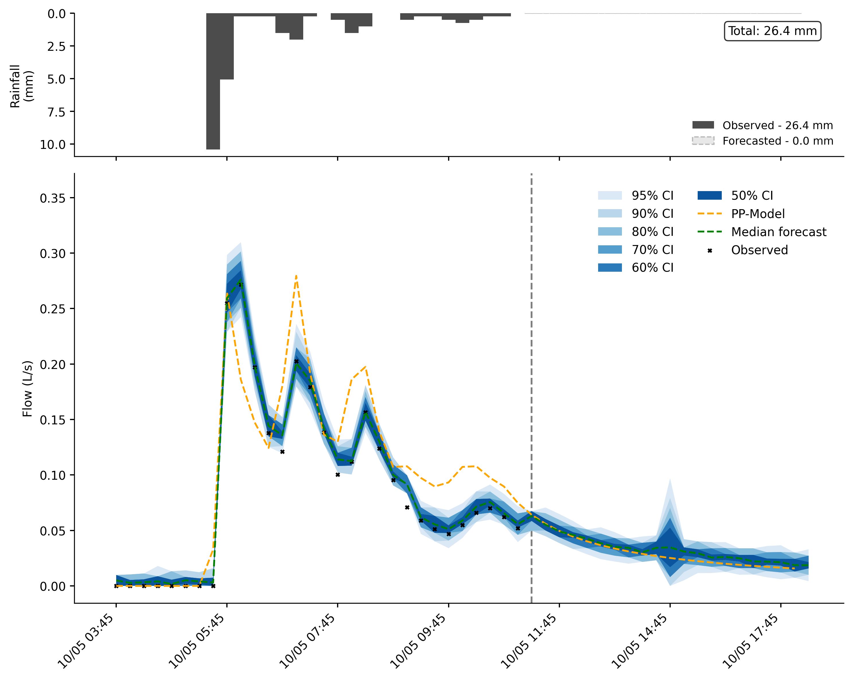
plot_output_path = os.path.join(base_dir, “output”, “particle_filter.png”) outflow_file_path = os.path.join(base_dir, “input”, “observed_outflow.ssv”)
metrics = plot_pp_forecast( results=results, forecast_time=30, plot_file=plot_output_path, obs_file=outflow_file_path, baseline_model_outflow=data[‘Qpipe’], rain_data=rain_data, date_series=data[‘date’], previous_forecast_data=None )
Result:
Summary
✅ Run basic water flow simulations ✅ Calibrate model parameters ✅ Download HRRR historical forecasts ✅ Perform particle filter forecasting
Get Help
Issues: GitHub Issues
Discussions: GitHub Discussions
Documentation: Continue reading these docs!
Happy modeling! 🌊